STAT 330 Lecture 31

Reading for Today's Lecture: 12.4, 12.5.

Goals of Today's Lecture:

• Learn to predict future Y values in simple linear regression.
• Learn the difference between estimating and predicting Y.
• Introduce sampling from the bivariate normal population.

Today's notes

Prediction Intervals: two problems to distinguish

1. Estimating the average Y value for a given x.
2. Predicting an individual Y value for a new value of x.

Notation:

• is a prediction of the Y value of a new individual.
• is the expected value of Y corresponding to a given x. For simple linear regression

  

We predict

by

• estimating and .
• predicting (because this is the mean of the population).

We get

Notice:

We can use these formulas to compute means and variances and then to get

• Confidence intervals for .
• Prediction intervals for Y.

Note: The uncertainty in guessing Y is much larger than that in guessing . Here is how to calculate these uncertainties.

This variance is big when x is far from and is always bigger than which is the value at .

and

The term 1 in [] is usually the big term in the sum.

Example: the burner data.

Returning to our example the fitted line is

and we have the following estimated standard errors:

Here are some predictions, standard errors of and Root mean squared prediction errors (which are estimates of the square root of ).

Std Err of RMS

x Pred Error

100 125 17 40

250 382 10 38

400 638 19 41

Note on alternative variance formulas. The following are all algebraically equivalent ways to compute :

Correlation Analysis

A different sort of bivariate data arises when the values of x cannot be controlled and instead we have a sample of pairs of numbers.

Our model will be that pairs

are sampled from a population of pairs.

Our analysis will be based on the assumption that the population distribution of these pairs is bivariate normal.

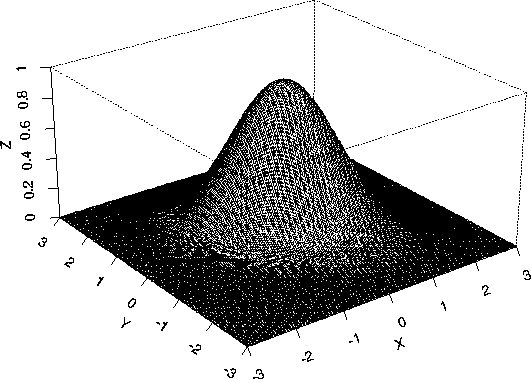
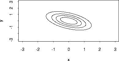
This means: That a three dimensional histogram (or the so called joint density of X and Y) would look like an elongated bell.

Another description can be obtained by drawing a contour plot of the density. The idea of a contour plot is that the density function f(x,y) describes the height of a surface at the point x,y. Imagine a rounded mountain like say Mount Seymour. If you had a vast saw and cut the top off the mountain the outline of the flat part would, for a bivariate normal density, be an ellipse. These outlines when the mountain is cut off at different heights are plotted below.

Properties of the bivariate normal density:

• If you imagine making a big vertical slice through this bell shaped mountain then the outline has the shape of a normal curve.
• For any constants a and b the variable aX+bY has a normal distribution.
• The bivariate normal density is specified by 5 parameters:
  • Two means: and which are the population means of X and Y.
  • Two standard deviations: and which are the population standard deviations of X and Y.
  • The Correlation Coefficient: