KALDFS Call

Language Reference

KALDFS Call

CALL KALDFS( sm, vsm, data, int, coef, var, bvec, bmat, initial, at,

mt, s2 <, un, vun>);

KALDFS computes the smoothed state vector and its mean square error matrix from the one-step forecast and mean square error matrix computed by KALDFF.

The inputs to the KALDFS subroutine are as follows:

data: is a T ×N_y matrix containing data (y₁, ... , y_T)'.
int: is an $(N_y + N_z) x N_\beta$ vector for a time-invariant intercept, or a $(T+{lead})(N_y + N_z) x N_\beta$ vector containing fixed matrices for the time-variant model in the transition equation and the measurement equation, that is, (W'_t, X'_t)'.
coef: is an (N_y + N_z) ×N_z matrix for a time-invariant coefficient, or a (T + lead)(N_y + N_z) ×N_z matrix containing coefficients at each time in the transition equation and the measurement equation, that is, (F'_t, H'_t)'.
var: is an (N_y + N_z) ×(N_y + N_z) matrix for a time-invariant variance matrix for transition equation noise and the measurement equation noise, or a (T + lead)(N_y + N_z) ×(N_y + N_z) matrix containing covariance matrices for the transition equation and measurement equation errors, that is, $(\eta^'_t, \epsilon^'_t)^'$ .
bvec: is an $N_\beta x 1$ constant vector for the intercept for the mean effect $\beta$ .
bmat: is an $N_\beta x N_\delta$ matrix for the coefficient for the mean effect $\beta$ .
initial: is an $N_\delta x (N_\delta + 1)$ matrix containing an initial random vector estimate and its covariance matrix, that is, $(\hat{\delta}_T, \hat{\Sigma}_\delta, T)$ .
at: is a $TN_z x (N_\delta + 1)$ matrix containing (A'₁, ... , A'_T)'.
mt: is a (TN_z) ×N_z matrix containing (M₁, ... , M_T)'.
s2: is the estimated variance in the end of the data set, $\hat{\sigma}^2_T$ .
un: is an optional $N_z x (N_{\delta} + 1)$ matrix containing ${\mu}_T$ . The returned value is ${\mu}_0$ .
vun: is an optional N_z ×N_z matrix containing U_T. The returned value is U₀.

The KALDFS call returns the following values:

sm: is a T ×N_z matrix containing smoothed state vectors $(z_{1| T}, ... , z_{T| T})^'$ .
vsm: is a TN_z ×N_z matrix containing mean square error matrices of smoothed state vectors $(P_{1| T}, ... , P_{T| T})^'$ .

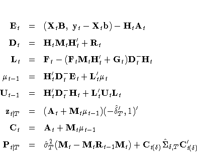
Given the one-step forecast and mean square error matrix in the KALDFF call, the KALDFS call computes a smoothed state vector and its mean square error matrix. Then the KALDFS subroutine produces an estimate of the smoothed state vector at time t, that is, the conditional expectation of the state vector z_t given all observations. Using the notations and results from the KALDFF section, the backward recursion algorithm for smoothing is denoted for t = T, T-1, ... , 1,

$E_t & = & (X_t B, y_t - X_t b) - H_t A_t \ D_t & = & H_t{M}_t{H}^'_t + R_t \ ... ..._t - M_t R_{t-1} M_t) + C_{t(\delta)} \hat{\Sigma}_{\delta,T} C^'_{t(\delta)}$

where the initial values are ${\mu}_T = 0$ and U_T = 0, and $C_{t(\delta)}$ is the last-column-deleted submatrix of C_t. Refer to De Jong (1991b) for details on smoothing in the diffuse Kalman filter.

The KALDFS call is accompanied by the KALDFF call as shown in the following code:

   ny = ncol(y);
   nz = ncol(coef);
   nb = ncol(int);
   nd = ncol(coefd);
   at = j(nz,nd+1,.);
   mt = j(nz,nz,.);
   qt = j(nd+1,nd+1,.);
   n0 = -1;
   call kaldff(pred,vpred,initial,s2,y,0,int,coef,var,intd,coefd,
               n0,at,mt,qt);
   bvec = intd[nz+1:nz+nb,];
   bmat = coefd[nz+1:nz+nb,];
   call kaldfs(sm,vsm,x,int,coef,var,bvec,bmat,initial,at,mt,s2);

You can also compute the smoothed estimate and its covariance matrix observation by observation. When the SSM is time invariant, the following code performs smoothing. You should initialize UN and VUN as matrices of value 0.

   n  = nrow(y);
   ny = ncol(y);
   nz = ncol(coef);
   nb = ncol(int);
   nd = ncol(coefd);
   at = j(nz,nd+1,.);
   mt = j(nz,nz,.);
   qt = j(nd+1,nd+1,.);
   n0 = -1;
   call kaldff(pred,vpred,initial,s2,y,0,int,coef,var,intd,coefd,
               n0,at,mt,qt);
   bvec = intd[nz+1:nz+nb,];
   bmat = coefd[nz+1:nz+nb,];
   un  = j(nz,nd+1,0);
   vun = j(nz,nz,0);
   do i = 1 to n;
      call kaldfs(sm_i,vsm_i,y[n-i+1],int,coef,var,bvec,bmat,
                  initial,at,mt,s2,un,vun);
      sm  = sm_i // sm;
      vsm = vsm_i // vsm;
   end;

Chapter Contents
Previous
Next
Top