The MODEL Procedure

Overview

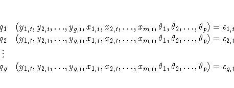
The MODEL procedure analyzes models in which the relationships among the variables comprise a system of one or more nonlinear equations. Primary uses of the MODEL procedure are estimation, simulation, and forecasting of nonlinear simultaneous equation models.

PROC MODEL features include

SAS programming statements to define simultaneous systems of nonlinear equations
tools to analyze the structure of the simultaneous equation system
ARIMA, PDL, and other dynamic modeling capabilities
tools to specify and estimate the error covariance structure
tools to estimate and solve ordinary differential equations
the following methods for parameter estimation:

-
Ordinary Least Squares (OLS)

-
Two-Stage Least Squares (2SLS)

-
Seemingly Unrelated Regression (SUR) and iterative SUR (ITSUR)

-
Three-Stage Least Squares (3SLS) and iterative 3SLS (IT3SLS)

-
Generalized Method of Moments (GMM)

-
Full Information Maximum Likelihood (FIML)
simulation and forecasting capabilities
Monte Carlo simulation
goal seeking solutions

A system of equations can be nonlinear in the parameters, nonlinear in the observed variables, or nonlinear in both the parameters and the variables. Nonlinear in the parameters means that the mathematical relationship between the variables and parameters is not required to have a linear form. (A linear model is a special case of a nonlinear model.) A general nonlinear system of equations can be written as

$&q_{1}&( y_{1,t}, y_{2,t} , { ... } , y_{g,t}, x_{1,t}, x_{2,t} , { ... } , x_{m... ...x_{m,t}, {\theta}_{1}, {\theta}_{2} , { ... } , {\theta}_{p}) = {\epsilon}_{g,t}$

where y_i,t is an endogenous variable, x_i,t is an exogenous variable, ${{\theta}_{i}}$ is a parameter, and ${{\epsilon}_{i}}$ is the unknown error. The subscript t represents time or some index to the data. In econometrics literature, the observed variables are either endogenous (dependent) variables or exogenous (independent) variables. This system can be written more succinctly in vector form as

$q( y_{t}, x_{t}, {{\theta}}) = {{\epsilon}}_{t}$

This system of equations is in general form because the error term is by itself on one side of the equality. Systems can also be written in normalized form by placing the endogenous variable on one side of the equality, with each equation defining a predicted value for a unique endogenous variable. A normalized form equation system can be written in vector notation as

$y_{t} = f( y_{t}, x_{t}, {{\theta}}) + {{\epsilon}}_{t}.$

PROC MODEL handles equations written in both forms.

Econometric models often explain the current values of the endogenous variables as functions of past values of exogenous and endogenous variables. These past values are referred to as lagged values, and the variable x_t-i is called lag i of the variable x_t. Using lagged variables, you can create a dynamic, or time dependent, model. In the preceding model systems, the lagged exogenous and endogenous variables are included as part of the exogenous variables.

If the data are time series, so that t indexes time (see chapter tsdata for more information on time series), it is possible that ${{{\epsilon}}_{t}}$ depends on ${{{\epsilon}}_{t-i}}$ or, more generally, the ${\epsilon}$ _t's are not identically and independently distributed. If the errors of a model system are autocorrelated, the standard error of the estimates of the parameters of the system will be inflated.

Sometimes the ${\epsilon}$ _i's are not identically distributed because the variance of ${\epsilon}$ is not constant. This is known as heteroscedasticity. Heteroscedasticity in an estimated model can also inflate the standard error of the estimates of the parameters. Using a weighted estimation can sometimes eliminate this problem. Alternately, a variance model such as GARCH or EGARCH can be estimated to correct for heteroscedasticity. If the proper weighting scheme and the form of the error model is difficult to determine, generalized methods of moments (GMM) estimation can be used to determine parameter estimates that are asymptotically more efficient than the OLS parameter estimates.

Other problems may also arise when estimating systems of equations. Consider the system of equations:

$y_{1,t} = {\theta}_{1} + ( {\theta}_{2} + {\theta}_{3} {\theta}^t_{4})^{-1} + {\theta}_{5}y_{2, t} + {\epsilon}_{1,t}$

$y_{2,t} = {\theta}_{6} + ( {\theta}_{7} + {\theta}_{8} {\theta}^t_{9})^{-1} + {\theta}_{10}y_{1, t}+ {\epsilon}_{2,t}$

which is nonlinear in its parameters and cannot be estimated with linear regression. This system of equations represents a rudimentary predator-prey process with y₁ as the prey and y₂ as the predator (the second term in both equations is a logistics curve). The two equations must be estimated simultaneously because of the cross dependency of y's. Nonlinear ordinary least-squares estimation of these equations will produce biased and inconsistent parameter estimates. This is called simultaneous equation bias.

One method to remove simultaneous equation bias, in the linear case, is to replace the endogenous variables on the right-hand side of the equations with predicted values that are uncorrelated with the error terms. These predicted values can be obtained through a preliminary, or "first stage," instrumental variable regression. Instrumental variables, which are uncorrelated with the error term, are used as regressors to model the predicted values. The parameter estimates are obtained by a second regression using the predicted values of the regressors. This process is called two-stage least squares.

In the nonlinear case, nonlinear ordinary least-squares estimation is performed iteratively using a linearization of the model with respect to the parameters. The instrumental solution to simultaneous equation bias in the nonlinear case is the same as the linear case except the linearization of the model with respect to the parameters is predicted by the instrumental regression. Nonlinear two-stage least squares is one of several instrumental variables methods available in the MODEL procedure to handle simultaneous equation bias.

When you have a system of several regression equations, the random errors of the equations can be correlated. In this case, the large-sample efficiency of the estimation can be improved by using a joint generalized least-squares method that takes the cross-equation correlations into account. If the equations are not simultaneous (no dependent regressors), then seemingly unrelated regression (SUR) can be used. The SUR method requires an estimate of the cross-equation error covariance matrix, ${\Sigma}$ .The usual approach is to first fit the equations using OLS, compute an estimate ${\hat{\Sigma}}$ from the OLS residuals, and then perform the SUR estimation based on ${\hat{\Sigma}}$ .The MODEL procedure estimates ${\Sigma}$ by default, or you can supply your own estimate of ${\Sigma}$ .

If the equation system is simultaneous, you can combine the 2SLS and SUR methods to take into account both simultaneous equation bias and cross-equation correlation of the errors. This is called three-stage least squares or 3SLS.

A different approach to the simultaneous equation bias problem is the full information maximum likelihood, or FIML, estimation method. FIML does not require instrumental variables, but it assumes that the equation errors have a multivariate normal distribution. 2SLS and 3SLS estimation do not assume a particular distribution for the errors.

Once a nonlinear model has been estimated, it can be used to obtain forecasts. If the model is linear in the variables you want to forecast, a simple linear solve can generate the forecasts. If the system is nonlinear, an iterative procedure must be used. The preceding example system is linear in its endogenous variables. The MODEL procedure's SOLVE statement is used to forecast nonlinear models.

One of the main purposes of creating models is to obtain an understanding of the relationship among the variables. There are usually only a few variables in a model you can control (for example, the amount of money spent on advertising). Often you want to determine how to change the variables under your control to obtain some target goal. This process is called goal seeking. PROC MODEL allows you to solve for any subset of the variables in a system of equations given values for the remaining variables.

The nonlinearity of a model creates two problems with the forecasts: the forecast errors are not normally distributed with zero mean, and no formula exits to calculate the forecast confidence intervals. PROC MODEL provides Monte Carlo techniques, which, when used with the covariance of the parameters and error covariance matrix, can produce approximate error bounds on the forecasts.

Chapter Contents
Previous
Next
Top