Lecture 7
Two Layer Artificial Neural Networks
Decision trees, while powerful, are a simple representation scheme. While graphical on the surface, they can be seen as disjunctions of conjunctions, and hence are a logical representation, and we call such schemes symbolic representations. In this lecture, we look at a non-symbolic representation scheme known as Artificial Neural Networks. This term is often shortened to Neural Networks, but this annoys neuro-biologists who deal with real neural networks (inside our human heads).
As the name suggests, ANNs have a biological motivation, and we briefly look at that first. Following this, we look in detail at how information is represented in ANNs, then we look at the simplest type of network, two layer networks. We look at perceptrons and linear units, and discuss the limitations that such simple networks have. In the next lecture, we discuss multi-layer networks and the back-propagation algorithm for learning such networks.
7.1 Biological Motivation
In our discussion in the first lecture about how people have answered the question: "How are we going to get an agent to act intelligently", one of the answers was to realise that intelligence in individual humans is effected by our brains. Neuro-scientists have told us that the brain is made up of architectures of networks of neurons. At the most basic level, neurons can be seen as functions which, when given some input, will either fire or not fire, depending on the nature of the input. The input to certain neurons comes from the senses, but in general, the input to a neuron is a set of outputs from other neurons. If the input to a neuron goes over a certain threshold, then the neuron will fire. In this way, one neuron firing will affect the firing of many other neurons, and information can be stored in terms of the thresholds set and the weight assigned by each neuron to each of its inputs.
Artificial Neural Networks (ANNs) are designed to mimic the behaviour of the brain. Some ANNs are built into hardware, but the vast majority are simulated in software, and we concentrate on these. It's important not to take the analogy too far, because there really isn't much similarity between artificial and animal neural networks. In particular, while the human brain is estimated to contain around 100,000,000,000 neurons, ANNs usually contain less than 1000 equivalent units. Moreover, the interconnection of neurons is much bigger in natural systems. Also, the way in which ANNs store and manipulate information is a gross simplification of the way in which networks of neurons work in natural systems.
7.2 ANN Representation
ANNs are taught on AI courses because of their motivation from brain studies and the fact that they are used in an AI task, namely machine learning. However, I would argue that their real home is in statistics, because, as a representation scheme, they are just fancy mathematical functions.
Imagine being asked to come up with a function to take the following inputs and produce their associated outputs:
| Input | Output |
| 1 | 1 |
| 2 | 4 |
| 3 | 9 |
| 4 | 16 |
Presumably, the function you would learn would be f(x) = x2. Imagine now that you had a set of values, rather than a single instance as input to your function:
| Input | Output |
| [1,2,3] | 1 |
| [2,3,4] | 5 |
| [3,4,5] | 11 |
| [4,5,6] | 19 |
Here, it is still possible to learn a function: for example, multiply the first and last element and take the middle one from the product. Note that the functions we are learning are getting more complicated, but they are still mathematical. ANNs just take this further: the functions they learn are generally so complicated that it's difficult to understand them on a global level. But they are still just functions which play around with numbers.
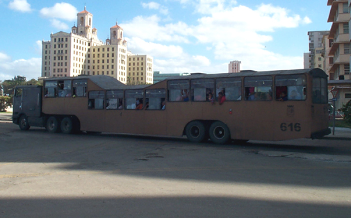
Imagine, now, for example, that the inputs to our function were arrays of pixels, actually taken from photographs of vehicles, and that the output of the function is either 1, 2 or 3, where 1 stands for a car, 2 stands for a bus and 3 stands for a tank:
| Input | Output | Input | Output |
 | 3 |  | 1 |
 | 2 |  | 1 |
In this case, the function which takes an array of integers representing pixel data and outputs either 1, 2 or 3 will be fairly complicated, but it's just doing the same kind of thing as the two simpler functions.
Because the functions learned to, for example, categorise photos of vehicles into a category of car, bus or tank, are so complicated, we say the ANN approach is a black box approach because, while the function performs well at its job, we cannot look inside it to gain a knowledge of how it works. This is a little unfair, as there are some projects which have addressed the problem of translating learned neural networks into human readable forms. However, in general, ANNs are used in cases where the predictive accuracy is of greater importance than understanding the learned concept.
Artificial Neural Networks consist of a number of units which are mini calculation devices. They take in real-valued input from multiple other nodes and they produce a single real valued output. By real-valued input and output we mean real numbers which are able to take any decimal value. The architecture of ANNs is as follows:
A set of input units which take in information about the example to be propagated through the network. By propagation, we mean that the information from the input will be passed through the network and an output produced. The set of input units forms what is known as the input layer.
-
A set of hidden units which take input from the input layer. The hidden units collectively form the hidden layer. For simplicity, we assume that each unit in the input layer is connected to each unit of the hidden layer, but this isn't necessarily the case. A weighted sum of the output from the input units forms the input to every hidden unit. Note that the number of hidden units is usually smaller than the number of input units.
A set of output units which, in learning tasks, dictate the category assigned to an example propagated through the network. The output units form the output layer. Again, for simplicity, we assume that each unit in the hidden layer is connected to each unit in the output layer. A weighted sum of the output from the hidden units forms the input to every output unit.
Hence ANNs look like this in the general case:
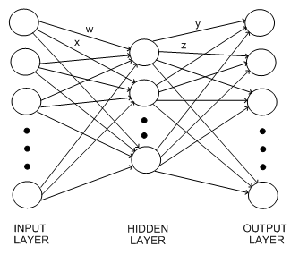
Note that the w, x, y and z represent real valued weights and that all the edges in this graph have weights associated with them (but it was difficult to draw them all on). Note also that more complicated ANNs are certainly possible. In particular, many ANNs have multiple hidden layers, with the output from one hidden layer forming the input to another hidden layer. Also, ANNs with no hidden layer - where the input units are connected directly to the output units - are possible. These tend to be too simple to use for real world learning problems, but they are useful to study for illustrative purposes, and we look at the simplest kind of neural networks, perceptrons, in the next section.
In our vehicle example, it is likely that the images will all be normalised to having the same number of pixels. Then there may be an input unit for each red, green and blue intensity for each pixel. Alternatively, greyscale images may be used, in which case there needs only to be an input node for each pixel, which takes in the brightness of the pixel. The hidden layer is likely to contain far fewer units (probably between 3 and 10) than the number of input units. The output layer will contain three units, one for each of the categories possible (car, bus, tank). Then, when the pixel data for an image is given as the initial values for the input units, this information will propagate through the network and the three output units will each produce a real value. The output unit which produces the highest value is taken as the categorisation for the input image.
So, for instance, when this image is used as input:
 |
then, if output unit 1 [car] produces value 0.5, output unit 2 [bus] produces value 0.05 and output unit 3 [tank] produces value 0.1, then this image has been (correctly) classified as a car, because the output from the corresponding car output unit is higher than for the other two. Exactly how the function embedded within a neural network computes the outputs given the inputs is best explained using example networks. In the next section, we look at the simplest networks of all, perceptrons, which consist of a set of input units connected to a single output unit.
7.3 Perceptrons
The weights in any ANN are always just real numbers and the learning problem boils down to choosing the best value for each weight in the network. This means there are two important decisions to make before we train a artificial neural network: (i) the overall architecture of the system (how input nodes represent given examples, how many hidden units/hidden layers to have and how the output information will give us an answer) and (ii) how the units calculate their real value output from the weighted sum of real valued inputs.
The answer to (i) is usually found by experimentation with respect to the learning problem at hand: different architectures are tried and evaluated on the learning problem until the best one emerges. In perceptrons, given that we have no hidden layer, the architecture problem boils down to just specifying how the input units represent the examples given to the network. The answer to (ii) is discussed in the next subsection.
- Units
The input units simply output the value which was input to them from the example to be propagated. Every other unit in a network normally has the same internal calculation function, which takes the weighted sum of inputs to it and calculates an output. There are different possibilities for the unit function and this dictates to some extent how learning over networks of that type is performed. Firstly, there is a simple linear unit which does no calculation, it just outputs the weighted sum which was input to it.
Secondly, there are other unit functions which are called threshold functions, because they are set up to produce low values up until the weighted sum reaches a particular threshold, then they produce high values after this threshold. The simplest type of threshold function produces a 1 if the weighted sum of the inputs is over a threshold value T, and produces a -1 otherwise. We call such functions step functions, due to the fact that, when drawn as a graph, it looks like a step. Another type of threshold function is called a sigma function, which has similarities with the step function, but advantages over it. We will look at sigma functions in the next lecture.
- Example
As an example, consider a ANN which has been trained to learn the following rule categorising the brightness of 2x2 black and white pixel images: if it contains 3 or 4 black pixels, it is dark; if it contains 2, 3 or 4 white pixels, it is bright. We can model this with a perceptron by saying that there are 4 input units, one for each pixel, and they output +1 if the pixel is white and -1 if the pixel is black. Also, the output unit produces a 1 if the input example is to be categorised as bright and -1 if the example is dark. If we choose the weights as in the following diagram, the perceptron will perfectly categorise any image of four pixels into dark or light according to our rule:
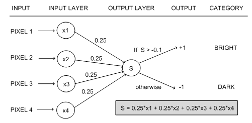
We see that, in this case, the output unit has a step function, with the threshold set to -0.1. Note that the weights in this network are all the same, which is not true in the general case. Also, it is convenient to make the weights going in to a node add up to 1, so that it is possible to compare them easily. The reason this network perfectly captures our notion of darkness and lightness is because, if three white pixels are input, then three of the input units produce +1 and one input unit produces -1. This goes into the weighted sum, giving a value of S = 0.25*1 + 0.25*1 + 0.25*1 + 0.25*(-1) = 0.5. As this is greater than the threshold of -0.1, the output node produces +1, which relates to our notion of a bright image. Similarly, four white pixels will produce a weighted sum of 1, which is greater than the threshold, and two white pixels will produce a sum of 0, also greater than the threshold. However, if there are three black pixels, S will be -0.5, which is below the threshold, hence the output node will output -1, and the image will be categorised as dark. Similarly, an image with four black pixels will be categorised as dark. As an exercise: keeping the weights the same, how low would the threshold have to be in order to misclassify an example with three or four black pixels?
- Learning Weights in Perceptrons
We will look in detail at the learning method for weights in multi-layer networks next lecture. The following description of learning in perceptrons will help clarify what is going on in the multi-layer case. We are in a machine learning setting, so we can expect the task to be to learn a target function which categorises examples into categories, given (at least) a set of training examples supplied with their correct categorisations. A little thought will be needed in order to choose the correct way of thinking about the examples as input to a set of input units, but, due to the simple nature of a perceptron, there isn't much choice for the rest of the architecture.
In order to produce a perceptron able to perform our categorisation task, we need to use the examples to train the weights between the input units and the output unit, and to train the threshold. To simplify the routine, we think of the threshold as a special weight, which comes from a special input node that always outputs a 1. So, we think of our perceptron like this:
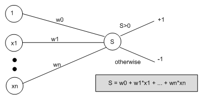
Then, we say that the output from the perceptron is +1 if the weighted sum from all the input units (including the special one) is greater than zero, and it outputs -1 otherwise. We see that weight w0 is simply the threshold value. However, thinking of the network like this means we can train w0 in the same way as we train all the other weights.
The weights are initially assigned randomly and training examples are used one after another to tweak the weights in the network. All the examples in the training set are used and the whole process (using all the examples again) is iterated until all examples are correctly categorised by the network. The tweaking is known as the perceptron training rule, and is as follows: If the training example, E, is correctly categorised by the network, then no tweaking is carried out. If E is mis-classified, then each weight is tweaked by adding on a small value, Δ. Suppose we are trying to calculate weight wi, which is between the i-th input unit, xi and the output unit. Then, given that the network should have calculated the target value t(E) for example E, but actually calculated the observed value o(E), then Δ is calculated as:
Δ = η (t(E)- o(E))xi
Note that η is a fixed positive constant called the learning rate. Ignoring η briefly, we see that the value Δ that we add on to our weight wi is calculated by multiplying the input value xi by t(E) - o(E). t(E) - o(E) will either be +2 or -2, because perceptrons output only +1 or -1, and t(E) cannot be equal to o(E), otherwise we wouldn't be doing any tweaking. So, we can think of t(E) - o(E) as a movement in a particular numerical direction, i.e., positive or negative. This direction will be such that, if the overall sum, S, was too low to get over the threshold and produce the correct categorisation, then the contribution to S from wi * xi will be increased. Conversely, if S is too high, the contribution from wi * xi is reduced. Because t(E) - o(E) is multiplied by xi, then if xi is a big value (positive or negative), the change to the weight will be greater. To get a better feel for why this direction correction works, it's a good idea to do some simple calculations by hand.
η simply controls how far the correction should go at one time, and is usually set to be a fairly low value, e.g., 0.1. The weight learning problem can be seen as finding the global minimum error, calculated as the proportion of mis-categorised training examples, over a space where all the input values can vary. Therefore, it is possible to move too far in a direction and improve one particular weight to the detriment of the overall sum: while the sum may work for the training example being looked at, it may no longer be a good value for categorising all the examples correctly. For this reason, η restricts the amount of movement possible. If a large movement is actually required for a weight, then this will happen over a series of iterations through the example set. Sometimes, η is set to decay as the number of such iterations through the whole set of training examples increases, so that it can move more slowly towards the global minimum in order not to overshoot in one direction. This kind of gradient descent is at the heart of the learning algorithm for multi-layered networks, as discussed in the next lecture.
Perceptrons with step functions have limited abilities when it comes to the range of concepts that can be learned, as discussed in a later section. One way to improve matters is to replace the threshold function with a linear unit, so that the network outputs a real value, rather than a 1 or -1. This enables us to use another rule, called the delta rule, which is also based on gradient descent. We don't look at this rule here, because the backpropagation learning method for multi-layer networks is similar.
7.4 Worked Example
Suppose we are trying to learn a perceptron to represent the brightness rules above, in such a way that if it outputs a 1, the image is categorised as bright, and if it outputs a -1, the image is categorised as dark. Remember that we said a 2x2 black and white pixel image is categorised as bright if it has two or more white pixels in it. We shall call the pixels p1 to p4, with the numbers going from left to right, top to bottom in the 2x2 image. A black pixel will produce an input of -1 to the network, and a white pixel will give an input of +1.
Given our new way of thinking about the threshold as a weight from a special input node, our network will have five input nodes and five weights. Suppose also that we have assigned the weights randomly to values between -1 and 1, namely -0.5, 0.7, -0.2, 0.1 and 0.9. Then our perceptron will initially look like this:
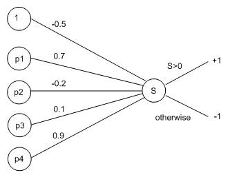
We will now train the network with the first training example, using a learning rate of η = 0.1. Suppose the first example image, E, is this:

With two white squares, this is categorised as bright. Hence, the target output for E is: t(E) = +1. Also, p1 (top left) is black, so the input x1 is -1. Similarly, x2 is +1, x3 is +1 and x4 is -1. Hence, when we propagate this through the network, we get the value:
S = (-0.5 * 1) + (0.7 * -1) + (-0.2 * +1) + (0.1 * +1) + (0.9 * -1) = -2.2
As this value is less than zero, the network outputs o(E) = -1, which is not the correct value. This means that we should now tweak the weights in light of the incorrectly categorised example. Using the perception training rule, we need to calculate the value of Δ to add on to each weight in the network. Plugging values into the formula for each weight gives us:
Δ0 = η (t(E)- o(E))xi = 0.1 * (1 - (-1)) * (1) = 0.1 * (2) = 0.2
Δ1 = η (t(E)- o(E))xi = 0.1 * (1 - (-1)) * (-1) = 0.1 * (-2) = -0.2
Δ2 = η (t(E)- o(E))xi = 0.1 * (1 - (-1)) * (1) = 0.1 * (2) = 0.2
Δ3 = η (t(E)- o(E))xi = 0.1 * (1 - (-1)) * (1) = 0.1 * (2) = 0.2
Δ4 = η (t(E)- o(E))xi = 0.1 * (1 - (-1)) * (-1) = 0.1 * (-2) = -0.2
When we add these values on to our existing weights, we get the new weights for the network as follows:
w'0 = -0.5 + Δ0 = -0.5 + 0.2 = -0.3
w'1 = 0.7 + Δ1 = 0.7 + -0.2 = 0.5
w'2 = -0.2 + Δ2 = -0.2 + 0.2 = 0
w'3 = 0.1 + Δ3 = 0.1 + 0.2 = 0.3
w'4 = 0.9 + Δ4 = 0.9 - 0.2 = 0.7
Our newly trained network will now look like this:
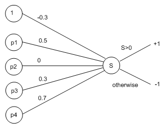
To see how this has improved the situation with respect to the training example, we can propagate it through the network again. This time, we get the weighted sum to be:
S = (-0.3 * 1) + (0.5 * -1) + (0 * +1) + (0.3 * +1) + (0.7 * -1) = -1.2
This is still negative, and hence the network categorises the example as dark, when it should be light. However, it is less negative. We can see that, by repeatedly training using this example, the training rule would eventually bring the network to a state where it would correctly categorise this example.
7.5 The Learning Abilities of Perceptrons
Computational learning theory is the study of what concepts particular learning schemes (representation and method) can and can't learn. We don't look at this in detail, but a famous example, first highlighted in a very influential book by Minsky and Papert involves perceptrons. It has been mathematically proven that the above method for learning perceptron weights will converge to a perfect classifier for learning tasks where the target concept is linearly separable.
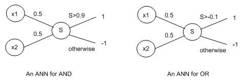
To understand what is and what isn't a linearly separable target function, we look at the simplest functions of all, boolean functions. These take two inputs, which are either 1 or -1 and output either a 1 or a -1. Note that, in other contexts, the values 0 and 1 are used instead of -1 and 1. As an example function, the AND boolean function outputs a 1 only if both inputs are 1, whereas the OR function only outputs a 1 if either inputs are 1. Obviously, these relate to the connectives we studied in first order logic. The following two perceptrons can represent the AND and OR boolean functions respectively:
One of the major impacts of Minsky and Papert's book was to highlight the fact that perceptrons cannot learn a particular boolean function called XOR. This function outputs a 1 if the two inputs are not the same. To see why XOR cannot be learned, try and write down a perceptron to do the job. The following diagram highlights the notion of linear separability in boolean functions, which explains why they can't be learned by perceptrons:
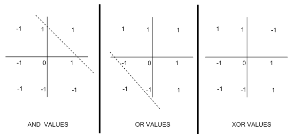
In each case, we've plotted the values taken by the boolean function when the inputs are particular values: (-1,-1);(1,-1);(-1,1) and (1,1). For the AND function, there is only one place where a 1 is plotted, namely when both inputs are 1. This meant that we could draw the dotted line to separate the output -1s from the 1s. We were able to draw a similar line in the OR case. Because we can draw these lines, we say that these functions are linearly separable. Note that it is not possible to draw such as line for the XOR plot: wherever you try, you never get a clean split into 1s and -1s.
The dotted lines can be seen as the threshold in perceptrons: if the weighted sum, S, falls below it, then the perceptron outputs one value, and if S falls above it, the alternative output is produced. It doesn't matter how the weights are organised, the threshold will still be a line on the graph. Therefore, functions which are not linearly separable cannot be represented by perceptrons.
Note that this result extends to functions over any number of variables, which can take in any input, but which produce a boolean output (and hence could, in principle be learned by a perceptron). For instance, in the following two graphs, the function takes in two inputs (like boolean functions), but the input can be over a range of values. The concept on the left can be learned by a perceptron, whereas the concept on the right cannot:
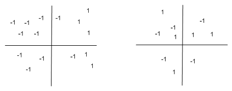
As an exercise, in the left hand plot, draw in the separating (threshold) line.
Unfortunately, the disclosure in Minsky and Papert's book that perceptrons cannot learn even such a simple function was taken the wrong way: people believed it represented a fundamental flaw in the use of ANNs to perform learning tasks. This led to a winter of ANN research within AI, which lasted over a decade. In reality, perceptrons were being studied in order to gain insights into more complicated architectures with hidden layers, which do not have the limitations that perceptrons have. No one ever suggested that perceptrons would be eventually used to solve real world learning problems. Fortunately, people studying ANNs within other sciences (notably neuro-science) revived interest in the study of ANNs. For more details of computational learning theory, see chapter 7 of Tom Mitchell's machine learning book.