Methodology and Spatial Analysis

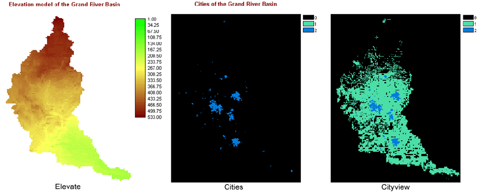
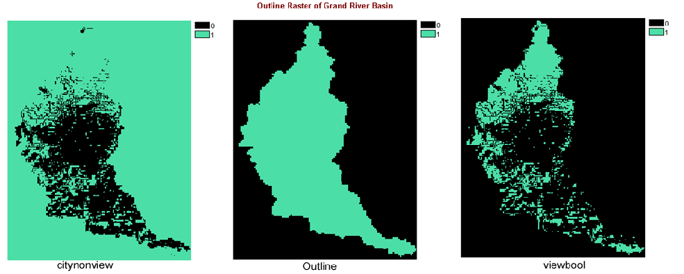
I then RE-CLASSED the layer cityview giving the area visible from the cities (and the cities) a value of 0 and the areas not visible from the cities a value of 1. This created the layer citynonview. I then used OVERLAY (First * Second) to combine the outline of the area with the citynonview layer in order to limit the possible areas to those I actually have data for and that are within the Grand River Basin; this created the layer viewbool (the two layers used to create this layer and the layer itself are provided below).
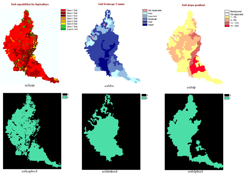
The next criteria used was to determine the area most likely to contain the commercially-viable tree species in the area (selected as eastern hemlock and eastern white pine). To do this I used data on the soils of the area to determine the areas most likely to contain these two tree species (both species having similar properties in terms of their ideal soils). I took the layer describing soil capabilities for agriculture, soilcap, and RE-CLASSED it to select the lowest two categories (Class 1 and Class 2 soils) as it in these areas that hemlock and pine are most competitive. I then RE-CLASSED the soil drainage layer, soildra, to select the moderate-to-rapid drainage areas. Finally I RE-CLASSED the soil slope gradient layer, soilslp, to select the areas with less than 10 degrees of soil slope. This created three boolean layers, soilcapbool, soildrabool and soilslpbool respectively (All six layers are provided below).
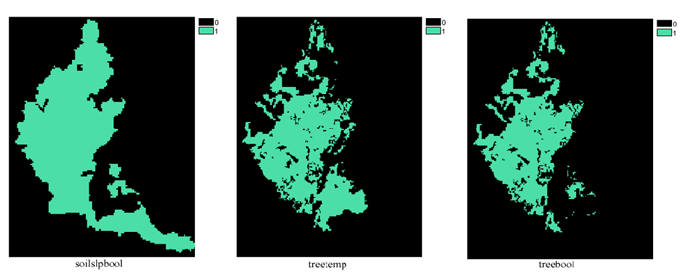
I then combined two of these boolean layers using the OVERLAY function (First * Second). In this case I combined soilcapbool and soildrabool to get the temporary layer treetemp. I then combined that layer with soilslpbool (again using OVERLAY First * Second) and created the layer treebool showing the area applying to all three tree soil criteria (all three layers pertaining to this step are again shown below).
Part 3: Woodlots/Boolean Combination
I already possessed a boolean layer showing the woodlots in the area, therefore I needed to combine it with the other boolean layers I created to provide the constraining area for my multiple-criteria evaluation. I combined the layers viewbool and treebool (the boolean layers created in the last two parts) to create the layer booltemp. I then combined that layer with woodlots and created the boolean layer boolfinal which combined all three criteria (all three layers used for this step are shown below).
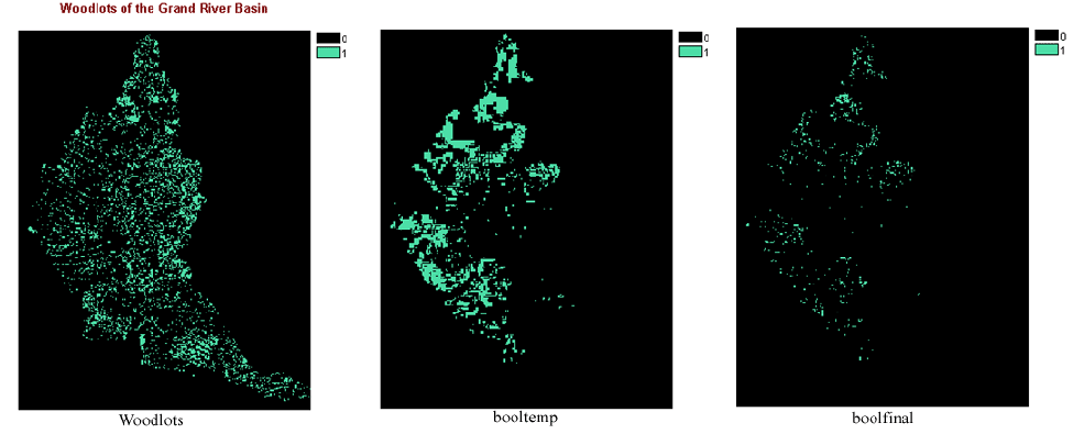
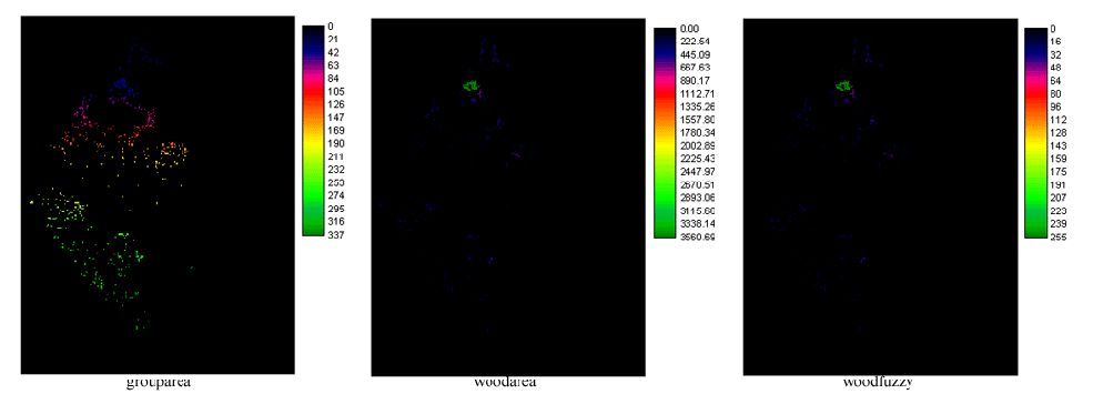
The first fuzzy criteria used for the analysis is the area of the woodlots in the area. Of course I only want to use those areas that apply to my boolean criteria since areas outside that would be useless for logging purposes, therefore I used the layer I created in the previous step, boolfinal, as the basis for this analysis. I used GROUP (use diagonals) to put all the pixels of boolfinal into groups and create the layer grouparea. I then used AREA to calculate the area of each group in acres to create the layer woodarea. Finally I used the FUZZY function to rate the areas in terms of their area (out of 256) using a linear increasing scale. I used 5 acres as the minimum area (a) and 3561 acres, the biggest area, as the maximum (b); this created the layer woodfuzzy. The layers created from GROUP, AREA and FUZZY are shown below.
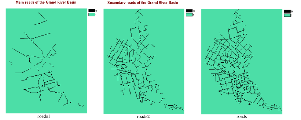
To find the distance from roads, I had to convert two vector layers, roads1 and roads2 (primary and secondary roads respectively), into two raster layers of the same name using the LINERAS function. These two raster layers then needed to be combined to form the overall road network of the area. I used OVERLAY (First * Second) to accomplish this and create the layer roads (these three layers are shown below).
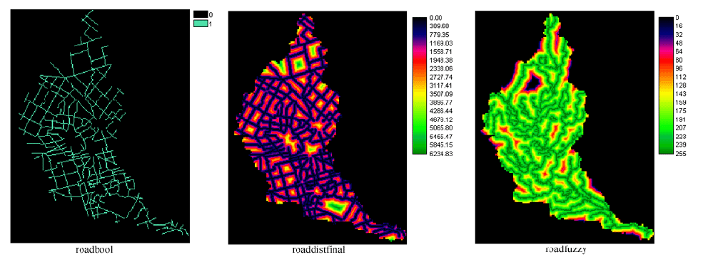
I then needed to RE-CLASS the roads layer to reverse the values and give the roads a value of 1 and the outside areas a value of 0. This RE-CLASS created the layer roadbool. I then used the DISTANCE function to create a layer, roaddist, showing the closest distance to a road of all the area of the Grand River Basin. I then combined this layer (using OVERLAY First * Second) with outline to create the image roaddistfinal to limit the layer to the areas within the Grand River Basin. Finally, I used the FUZZY function to assign values (out of 256) based on the pixels' distances from roads. I used the linear decreasing function (since the logging operation would like to be as close to a road as possible) and used 6,235 meters, the highest value, as the maximum (c) and 0 meters as the minimum (d). This created the layer roadfuzzy (images pertaining to these operations are shown below).
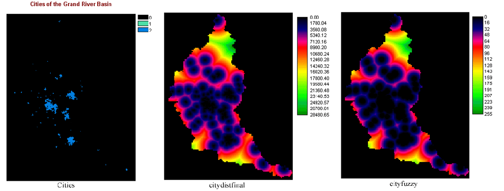
The next criteria used was the distance to cities. I took the layer cities and using the DISTANCE function to create a layer, citydist, showing the distance all the pixels are from a major city. I then used OVERLAY (First * Second) with outline again to limit the possible area to that within the Grand River Basin creating the layer citydistfinal. Finally I used the FUZZY function to assign values (out of 256) using a linear increasing function to each pixel based on their distance from cities. I used a minimum value (a) of 2000 meters and a maximum value (b), the highest pixel value, of 28,481 meters. This created the layer cityfuzzy (three layers from this part are shown below).
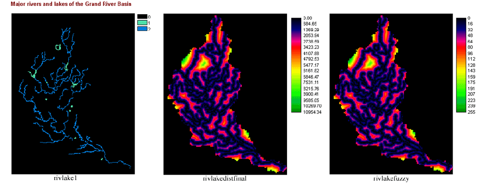
The final criteria used to find the ideal logging site is the distance from rivers and lakes. First I had to RE-CLASS the layer rivlake1 in order to create a boolean image, rivlake, simply giving all water bodies a value of 1 and all other areas a value of 0. I then used the DISTANCE function to create a layer, rivlakedist, showing the distance each pixel is from a river or lake. I then combined that layer with outline again to limit the possible areas to those within the Grand River Basin; this created the layer rivlakedistfinal. Finally, I used the FUZZY function to assign values (out of 256) to each pixel based on their distances from rivers and lakes. I used a linear increasing function and used 55 meters (the environmental standard) as a, the minimum value and 10,955 meters (the highest pixel value) as b, the maximum value. This created the layer rivlakefuzzy (Three images pertaining to this part provided below).
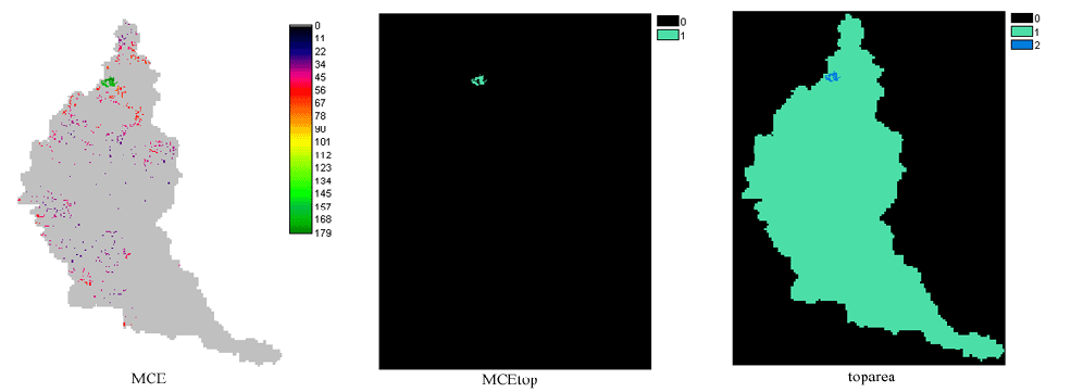
I then, to find the actual results of my analysis, had to combine all the fuzzy parameters together using a multiple-criteria evaluation (MCE). I therefore used the MCE function. Using this function I created a weighted linear combination of the four fuzzy layers I had previously created, using the layer boolfinal as a constraining area. I weighted the layers based on their importance to the logging company. The wood area (woodfuzzy) was most important at 0.45 as this determined how much money the company could make. Next was the distance from rivers and lakes (rivlakefuzzy) at 0.25 to keep the environmentalists happy. Third the distance from cities (cityfuzzy) at 0.20; this value would have been much higher but since areas within view of cities were already eliminated there would not be many resulting areas near cities. The final factor used was the distance to roads (roadfuzzy) at 0.10; this value is the lowest because though it would be more convenient and save the company some money, the company is used to building their own roads and do not consider this factor extremely important in site selection. This analysis created the layer MCE (shown with a grey background so the areas stand out better). One area stands out with a much higher value than all the others. I isolated it as the ideal area using RE-CLASS to select only the areas with values over 160 and created the layer MCEtop. I then combined this layer using OVERLAY (First + Second) with outline to create the layer toparea which shows the top area for logging based on my analysis displayed on the background of the outline of the Grand River Basin.
Back to Top | Back to Main Menu | Previous Page | Next Page