Spatial Analysis -- Raw Data Analysis
The following are steps of our raw data analysis:
Postal code
The 6 digit postal code data had many duplicate postal codes for the purposes of corresponding with the Canadian Senses data. The Canadian Census has a tool called “Postal2Census” which was used to associate historic census geography boundaries (UEP) with Canadian postal code points (MEP) (StatsCan, 2006). Therefore all postal code areas with the same postal code name were merged together to eliminate any duplicate names.
Population density
The smaller the area, the more chances that density measures can get skewed because density is a function of area size. Therefore, when measuring population density of 6-digit postal codes, the measures had to be normalised. The original Canada Census data are in a unit of Dissemination Areas. We spatial join those areas with 6 digit postal code areas. The steps to analyze population density were coded as follows:
- Start with ‘Census population’ dataset.
- Clip the dataset to 6-digit postal code boundaries.
- Spatially Join the two data sets together.
- Calculate density by dividing the population by areas.
- Normalise data.
- Rank from 1 to 5: 1 representing very dense/walkable and 5 representing not dense at all/not walkable.

Street network
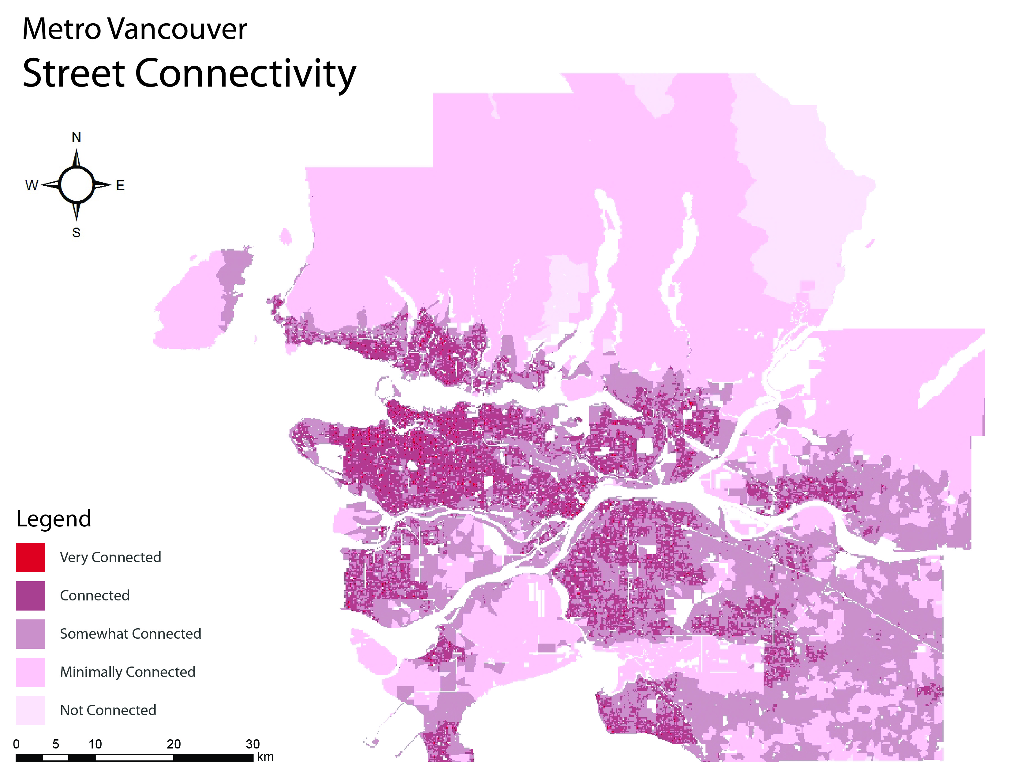
The ‘Street Network’ dataset was given a 2 meter buffer to ensure roads that bordered the postal codes boundaries were included in the connectivity of both postal codes. The data was classified and ranked into 5 ranks of connectivity: 1 representing very connected/walkable and 5 representing not connected at all/not walkable. The steps to analyze connectivity were coded as follows:
- Start with ‘6-digit postal code’ dataset.
- Add a 2 meter buffer to the ‘Road Network’ dataset.
- Run Spatial Join to join both datasets and count roads per 6-digit postal code
- Create a proportion based on number of roads per area
- Normalise data to avoid skewness.
- Rank from 1 to 5: 1 representing very connected/walkable and 5 representing not connected at all/not walkable.

Transit stops
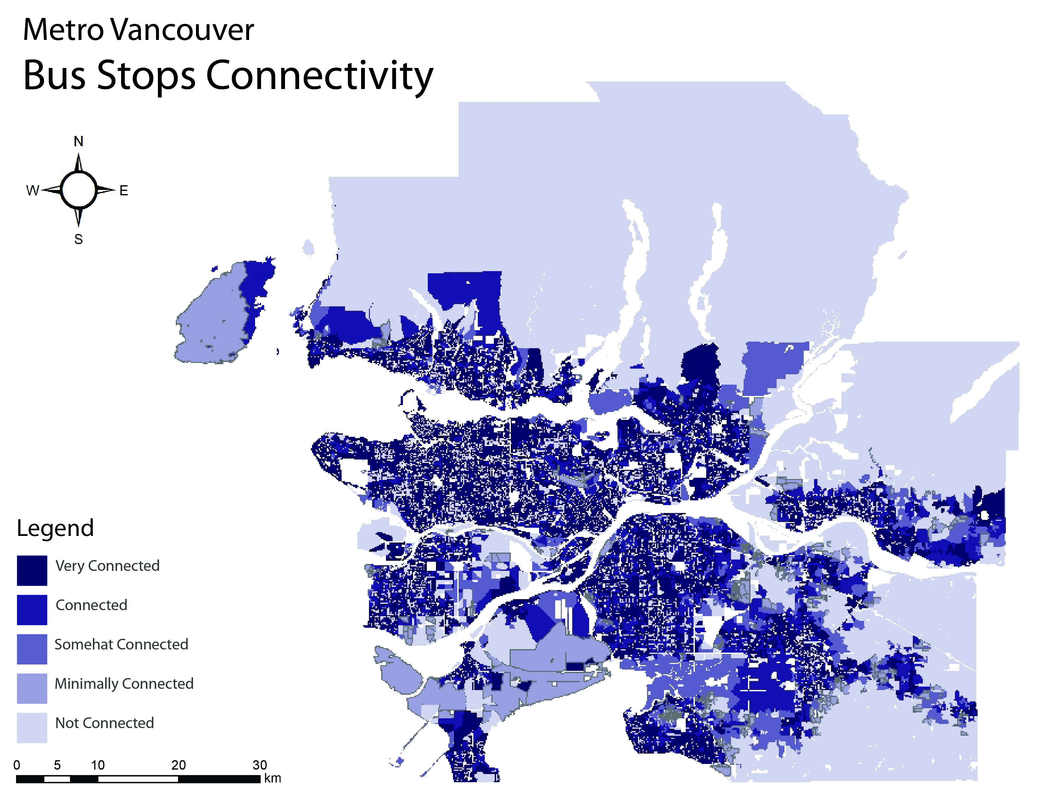
In order to create a route from the centroid of a 6-digit postal code to the nearest transit stop, a network dataset needed to be created from the ‘Road Network’ dataset. The network analyst tools were able to accurately draw routes with a buffer specification of 2km for this analysis. The steps to analyze connectivity to transit stops were coded as follows:
- Start with ‘road network’ dataset.
- Create network dataset from ‘road network’ dataset.
- Run ‘closest facility’ network analysis from centroid of postal codes to the nearest transit stops and measure distance.
- Create a proportion based on number of roads per area.
- Multiply distance by walk speed using field calculator.
- Rank from 1 to 5: 1 representing very connected/walkable and 5 representing not connected at all/not walkable.

Land use data
The land use data collected from Metro Vancouver included land use mix metadata that was useful to walkability research. The 16 land use classes included in the data were narrowed down to include the following: commercial, all types of residential uses, commercial-residential mixed, institutional, recreation and naturally protected areas, lakes and water bodies. The steps to analyze land use mix were coded as follows:
- Start with the Metro Vancouver ‘land use mix’ dataset.
- Dissolve the land use areas together.
- Run a spatial join to join land use with FSA boundaries.
- Create a count of land use categories per FSA.
- Rank from 1 to 5: 1 representing very mixed/walkable and 5 representing not mixed at all/not walkable.

Park location data
Very similar to the distance to transit stops, the distance to parks was analyzed using the ‘Closest Facility’ Network Analyst. The steps to analyze distance to parks were coded as follows:
- Start with ‘land use’ dataset.
- Crop ‘recreation and protected natural areas’ from ‘land use’ into a new shapefile called ‘parks’.
- Run ‘closest facility’ layer using the previously created ‘road network’ from centroid of postal code to nearest park and measure distance.
- Convert distance to cut-off value using field calculator.
- Rank from 1 to 5: 1 representing very accessible/walkable and 5 representing not accessible at all/not walkable.

Metro Vancouver Digital Elevation Model (DEM)
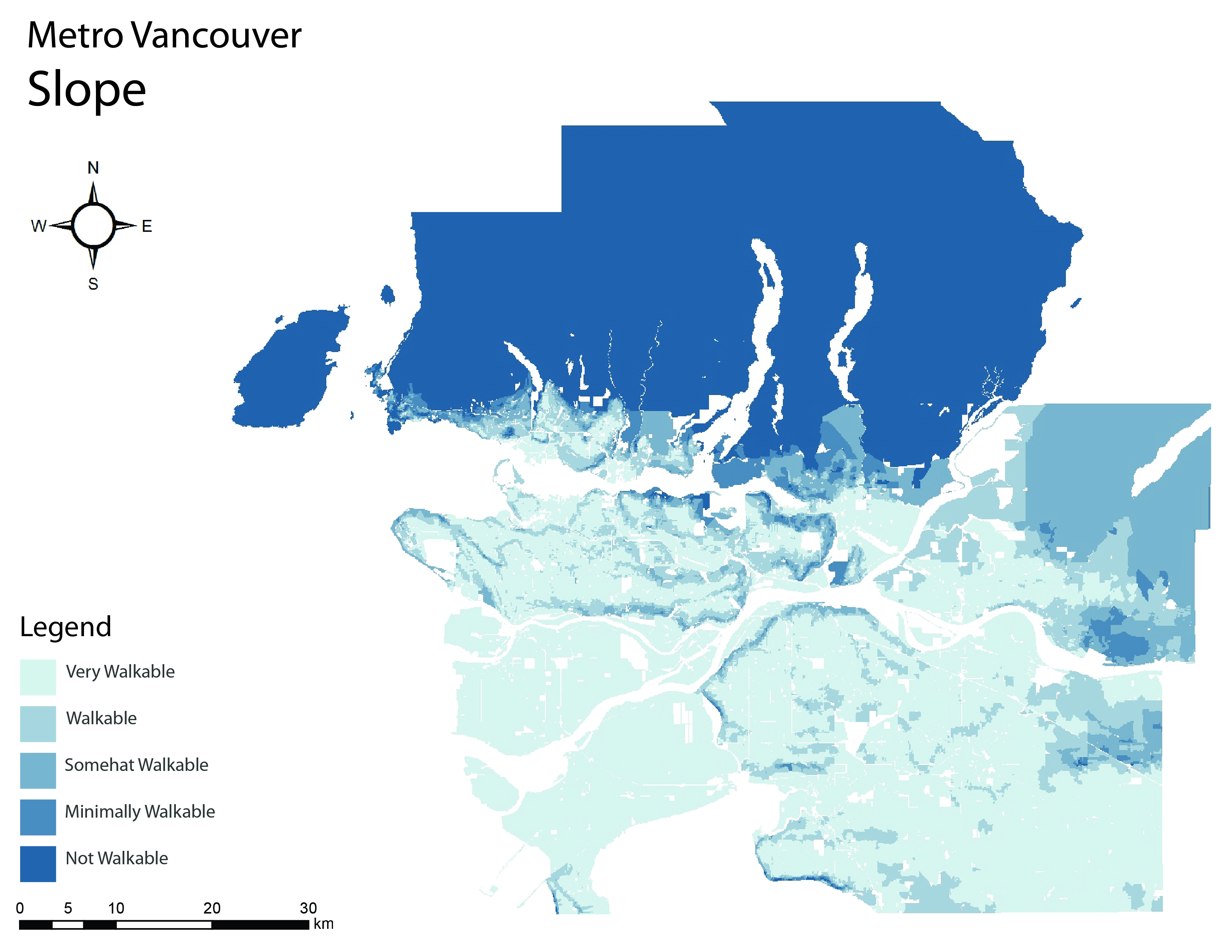
In order to accurately convert the DEM slope dataset from raster to vector several steps had to be followed that aren’t listed here in detail. However, in order to maintain a high standard of data preservation, a spatial join was run in order to average the slope per postal code boundary. The steps to analyze slope were coded as follows:
- Start with DEM of Metro Vancouver
- Create a zonal statistics map using the vector 6-digit postal code boundaries.
- Use the INT function to convert the float data attributes into integer data attribute.
- Convert the zonal statistics raster map into vector map.
- Run Spatial Join to join postal code data and the zonal statistic data.
- Rank from 1 to 5: 1 representing very walkable and 5 representing not walkable.

Vancouver Area Neighbourhood Deprivation Index (VANDIX)
VANDIX data represents socioeconomic data in our research and was joined to the 6-digit postal code data. There are 21 Variables for measuring VANDIX which were all relabeled into 7 categories and joined to the 6-digit postal code data. The preparaion steps of VANDIX are as follows, for further use of VANDIX, please see Secondary Analysis.
- Run Spatial Join to join VANDIX with 6-digit postal code
- Rank from 1 to 5: 1 representing very safe/walkable and 5 representing not safe at all/not walkable.