Lecture 8
Multi-Layer Artificial Neural Networks
We can now look at more sophisticated ANNs, which are known as multi-layer artificial neural networks because they have hidden layers. These will naturally be used to undertake more complicated tasks than perceptrons. We first look at the network structure for multi-layer ANNs, and then in detail at the way in which the weights in such structures can be determined to solve machine learning problems. There are many considerations involved with learning such ANNs, and we consider some of them here. First and foremost, the algorithm can get stuck in local minima, and there are some ways to try to get around this. As with any learning technique, we will also consider the problem of overfitting, and discuss which types of problems an ANN approach is suitable for.
8.1 Multi-Layer Network Architectures
We saw in the previous lecture that perceptrons have limited scope in the type of concepts they can learn - they can only learn linearly separable functions. However, we can think of constructing larger networks by building them out of perceptrons. In such larger networks, we call the step function units the perceptron units in multi-layer networks.
As with individual perceptrons, multi-layer networks can be used for learning tasks. However, the learning algorithm that we look at (the backpropagation routine) is derived mathematically, using differential calculus. The derivation relies on having a differentiable threshold function, which effectively rules out using perceptron units if we want to be sure that backpropagation works correctly. The step function in perceptrons is not continuous, hence non-differentiable. An alternative unit was therefore chosen which had similar properties to the step function in perceptron units, but which was differentiable. There are many possibilities, one of which is sigmoid units, as described below.
- Sigmoid units
Remember that the function inside units take as input the weighted sum, S, of the values coming from the units connected to it. The function inside sigmoid units calculates the following value, given a real-valued input S:
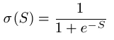
Where e is the base of natural logarithms, e = 2.718...
When we plot the output from sigmoid units given various weighted sums as input, it looks remarkably like a step function:
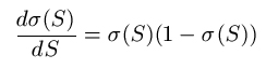
Of course, getting a differentiable function which looks like the step function was the whole point of the exercise. In fact, not only is this function differentiable, but the derivative is fairly simply expressed in terms of the function itself:
Note that the output values for the σ function range between but never make it to 0 and 1. This is because e-S is never negative, and the denominator of the fraction tends to 0 as S gets very big in the negative direction, and tends to 1 as it gets very big in the positive direction. This tendency happens fairly quickly: the middle ground between 0 and 1 is rarely seen because of the sharp (near) step in the function. Because of it looking like a step function, we can think of it firing and not-firing as in a perceptron: if a positive real is input, the output will generally be close to +1 and if a negative real is input the output will generally be close to -1.
- Example Multi-layer ANN with Sigmoid Units
We will concern ourselves here with ANNs containing only one hidden layer, as this makes describing the backpropagation routine easier. Note that networks where you can feed in the input on the left and propagate it forward to get an output are called feed forward networks. Below is such an ANN, with two sigmoid units in the hidden layer. The weights have been set arbitrarily between all the units.
Note that the sigma units have been identified with sigma signs in the node on the graph. As we did with perceptrons, we can give this network an input and determine the output. We can also look to see which units "fired", i.e., had a value closer to 1 than to 0.
Suppose we input the values 10, 30, 20 into the three input units, from top to bottom. Then the weighted sum coming into H1 will be:
SH1 = (0.2 * 10) + (-0.1 * 30) + (0.4 * 20) = 2 -3 + 8 = 7.
Then the σ function is applied to SH1 to give:
σ(SH1) = 1/(1+e-7) = 1/(1+0.000912) = 0.999
[Don't forget to negate S]. Similarly, the weighted sum coming into H2 will be:
SH2 = (0.7 * 10) + (-1.2 * 30) + (1.2 * 20) = 7 - 36 + 24 = -5
and σ applied to SH2 gives:
σ(SH2) = 1/(1+e5) = 1/(1+148.4) = 0.0067
From this, we can see that H1 has fired, but H2 has not. We can now calculate that the weighted sum going in to output unit O1 will be:
SO1 = (1.1 * 0.999) + (0.1*0.0067) = 1.0996
and the weighted sum going in to output unit O2 will be:
SO2 = (3.1 * 0.999) + (1.17*0.0067) = 3.1047
The output sigmoid unit in O1 will now calculate the output values from the network for O1:
σ(SO1) = 1/(1+e-1.0996) = 1/(1+0.333) = 0.750
and the output from the network for O2:
σ(SO2) = 1/(1+e-3.1047) = 1/(1+0.045) = 0.957
Therefore, if this network represented the learned rules for a categorisation problem, the input triple (10,30,20) would be categorised into the category associated with O2, because this has the larger output.
8.2 The Backpropagation Learning Routine
As with perceptrons, the information in the network is stored in the weights, so the learning problem comes down to the question: how do we train the weights to best categorise the training examples. We then hope that this representation provides a good way to categorise unseen examples.
In outline, the backpropagation method is the same as for perceptrons:
- We choose and fix our architecture for the network, which
will contain input, hiddedn and output units, all of which will contain
sigmoid functions.
We randomly assign the weights between all the nodes. The assignments should be to small numbers, usually between -0.5 and 0.5.
-
Each training example is used, one after another, to re-train the weights in the network. The way this is done is given in detail below.
-
After each epoch (run through all the training examples), a termination condition is checked (also detailed below). Note that, for this method, we are not guaranteed to find weights which give the network the global minimum error, i.e., perfectly correct categorisation of the training examples. Hence the termination condition may have to be in terms of a (possibly small) number of mis-categorisations. We see later that this might not be such a good idea, though.
- Weight Training Calculations
Because we have more weights in our network than in perceptrons, we firstly need to introduce the notation: wij to specify the weight between unit i and unit j. As with perceptrons, we will calculate a value Δij to add on to each weight in the network after an example has been tried. To calculate the weight changes for a particular example, E, we first start with the information about how the network should perform for E. That is, we write down the target values ti(E) that each output unit Oi should produce for E. Note that, for categorisation problems, ti(E) will be zero for all the output units except one, which is the unit associated with the correct categorisation for E. For that unit, ti(E) will be 1.
Next, example E is propagated through the network so that we can record all the observed values oi(E) for the output nodes Oi. At the same time, we record all the observed values hi(E) for the hidden nodes. Then, for each output unit Ok, we calculate its error term as follows:

The error terms from the output units are used to calculate error terms for the hidden units. In fact, this method gets its name because we propagate this information backwards through the network. For each hidden unit Hk, we calculate the error term as follows:
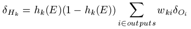
In English, this means that we take the error term for every output unit and multiply it by the weight from hidden unit Hk to the output unit. We then add all these together and multiply the sum by hk(E)*(1 - hk(E)).
Having calculated all the error values associated with each unit (hidden and output), we can now transfer this information into the weight changes Δij between units i and j. The calculation is as follows: for weights wij between input unit Ii and hidden unit Hj, we add on:
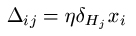
[Remembering that xi is the input to the i-th input node for example E; that η is a small value known as the learning rate and that δHj is the error value we calculated for hidden node Hj using the formula above].
For weights wij between hidden unit Hi and output unit Oj, we add on:
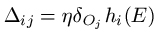
[Remembering that hi(E) is the output from hidden node Hi when example E is propagated through the network, and that δOj is the error value we calculated for output node Oj using the formula above].
Each alteration Δ is added to the weights and this concludes the calculation for example E. The next example is then used to tweak the weights further. As with perceptrons, the learning rate is used to ensure that the weights are only moved a short distance for each example, so that the training for previous examples is not lost. Note that the mathematical derivation for the above calculations is based on derivative of σ that we saw above. For a full description of this, see chapter 4 of Tom Mitchell's book "Machine Learning".
8.3 A Worked Example
We will re-use the example from section 8.1, where our network originally looked like this:
and we propagated the values (10,30,20) through the network. When we did so, we observed the following values:
| Input units | Hidden units | Output units | |||||
| Unit | Output | Unit | Weighted Sum Input | Output | Unit | Weighted Sum Input | Output |
| I1 | 10 | H1 | 7 | 0.999 | O1 | 1.0996 | 0.750 |
| I2 | 30 | H2 | -5 | 0.0067 | O2 | 3.1047 | 0.957 |
| I3 | 20 | ||||||
Suppose now that the target categorisation for the example was the one associated with O1. This means that the network mis-categorised the example and gives us an opportunity to demonstrate the backpropagation algorithm: we will update the weights in the network according to the weight training calculations provided above, using a learning rate of η = 0.1.
If the target categorisation was associated with O1, this means that the target output for O1 was 1, and the target output for O2 was 0. Hence, using the above notation,
t1(E) = 1; t2(E) = 0; o1(E) = 0.750; o2(E) = 0.957
That means we can calculate the error values for the output units O1 and O2 as follows:
δO1 = o1(E)(1 - o1(E))(t1(E) - o1(E)) = 0.750(1-0.750)(1-0.750) = 0.0469
δO2 = o2(E)(1 - o2(E))(t2(E) - o2(E)) = 0.957(1-0.957)(0-0.957) = -0.0394
We can now propagate this information backwards to calculate the error terms for the hidden nodes H1 and H2. To do this for H1, we multiply the error term for O1 by the weight from H1 to O1, then add this to the multiplication of the error term for O2 and the weight between H1 and O2. This gives us: (1.1*0.0469) + (3.1*-0.0394) = -0.0706. To turn this into the error value for H1, we multiply by h1(E)*(1-h1(E)), where h1(E) is the output from H1 for example E, as recorded in the table above. This gives us:
δH1 = -0.0706*(0.999 * (1-0.999)) = -0.0000705
A similar calculation for H2 gives the first part to be: (0.1*0.0469)+(1.17*-0.0394) = -0.0414, and the overall error value to be:
δH2 -0.0414 * (0.067 * (1-0.067)) = -0.00259
We now have all the information required to calculate the weight changes for the network. We will deal with the 6 weights between the input units and the hidden units first:
| Input unit | Hidden unit | η | δH | xi | Δ = η*δH*xi | Old weight | New weight |
| I1 | H1 | 0.1 | -0.0000705 | 10 | -0.0000705 | 0.2 | 0.1999295 |
| I1 | H2 | 0.1 | -0.00259 | 10 | -0.00259 | 0.7 | 0.69741 |
| I2 | H1 | 0.1 | -0.0000705 | 30 | -0.0002115 | -0.1 | -0.1002115 |
| I2 | H2 | 0.1 | -0.00259 | 30 | -0.00777 | -1.2 | -1.20777 |
| I3 | H1 | 0.1 | -0.0000705 | 20 | -0.000141 | 0.4 | 0.39999 |
| I3 | H2 | 0.1 | -0.00259 | 20 | -0.00518 | 1.2 | 1.1948 |
We now turn to the problem of altering the weights between the hidden layer and the output layer. The calculations are similar, but instead of relying on the input values from E, they use the values calculated by the sigmoid functions in the hidden nodes: hi(E). The following table calculates the relevant values:
| Hidden unit |
Output unit |
η | δO | hi(E) | Δ = η*δO*hi(E) | Old weight | New weight |
| H1 | O1 | 0.1 | 0.0469 | 0.999 | 0.000469 | 1.1 | 1.100469 |
| H1 | O2 | 0.1 | -0.0394 | 0.999 | -0.00394 | 3.1 | 3.0961 |
| H2 | O1 | 0.1 | 0.0469 | 0.0067 | 0.00314 | 0.1 | 0.10314 |
| H2 | O2 | 0.1 | -0.0394 | 0.0067 | -0.0000264 | 1.17 | 1.16998 |
We note that the weights haven't altered all that much, so it might be a good idea in this situation to use a bigger learning rate. However, remember that, with sigmoid units, small changes in the weighted sum can produce big changes in the output from the unit.
As an exercise, check whether the re-trained network performs better with respect to the example than the original network.
8.4 Avoiding Local Minima
The error rate of multi-layered networks over a training set could be calculated as the number of mis-classified examples. Remembering, however, that there are many output nodes, all of which could potentially misfire (e.g., giving a value close to 1 when it should have output 0, and vice-versa), we can be more sophisticated in our error evaluation. In practice the overall network error is calculated as:
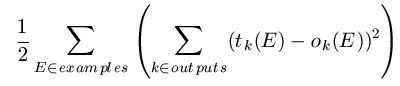
This is not as complicated as it first appears. The calculation simply involves working out the difference between the observed output for each output unit and the target output and squaring this to make sure it is positive, then adding up all these squared differences for each output unit and for each example.
Backpropagation can be seen as using searching a space of network configurations (weights) in order to find a configuration with the least error, measured in the above fashion. The more complicated network structure means that the error surface which is searched can have local minima, and this is a problem for multi-layer networks, and we look at ways around it below. Having said that, even if a learned network is in a local minima, it may still perform adequately, and multi-layer networks have been used to great effect in real world situations (see Tom Mitchell's book for a description of an ANN which can drive a car!)
One way around the problem of local minima is to use random re-start as described in the lecture on search techniques. Different initial random weightings for the network may mean that it converges to different local minima, and the best of these can be taken for the learned ANN. Alternatively, as described in Mitchell's book, a "committee" of networks could be learned, with the (possibly weighted) average of their decisions taken as an overall decision for a given test example. Another alternative is to try and skip over some of the smaller local minima, as described below.
- Adding Momentum
Imagine a ball rolling down a hill. As it does so, it gains momentum, so that its speed increases and it becomes more difficult to stop. As it rolls down the hill towards the valley floor (the global minimum), it might occasionally wander into local hollows. However, it may be that the momentum it has obtained keeps it rolling up and out of the hollow and back on track to the valley floor.
The crude analogy describes one heuristic technique for avoiding local minima, called adding momentum, funnily enough. The method is simple: for each weight remember the previous value of Δ which was added on to the weight in the last epoch. Then, when updating that weight for the current epoch, add on a little of the previous Δ. How small to make the additional extra is controlled by a parameter α called the momentum, which is set to a value between 0 and 1.
To see why this might help bypass local minima, note that if the weight change carries on in the direction it was going in the previous epoch, then the movement will be a little more pronounced in the current epoch. This effect will be compounded as the search continues in the same direction. When the trend finally reverses, then the search may be at the global minimum, in which case it is hoped that the momentum won't be enough to take it anywhere other than where it is. Alternatively, the search may be at a fairly narrow local minimum. In this case, even though the backpropagation algorithm dictates that Δ will change direction, it may be that the additional extra from the previous epoch (the momentum) may be enough to counteract this effect for a few steps. These few steps may be all that is needed to bypass the local minimum.
In addition to getting over some local minima, when the gradient is constant in one direction, adding momentum will increase the size of the weight change after each epoch, and the network may converge quicker. Note that it is possible to have cases where (a) the momentum is not enough to carry the search out of a local minima or (b) the momentum carries the search out of the global minima into a local minima. This is why this technique is a heuristic method and should be used somewhat carefully (it is used in practice a great deal).
8.5 Overfitting Considerations
Left unchecked, backpropagation in multi-layer networks can be highly susceptible to overfitting itself to the training examples. The following graph plots the error on the training and test set as the number of weight updates increases. It is typical of networks left to train unchecked.
Alarmingly, even though the error on the training set continues to gradually decrease, the error on the test set actually begins to increase towards the end. This is clearly overfitting, and it relates to the network beginning to find and fine-tune to ideosyncrasies in the data, rather than to general properties. Given this phenomena, it would be unwise to use some kind of threshold for the error as the termination condition for backpropagation.
In cases where the number of training examples is high, one antidote to overfitting is to split the training examples into a set to use to train the weight and a set to hold back as an internal validation set. This is a mini-test set, which can be used to keep the network in check: if the error on the validation set reaches a minima and then begins to increase, then it could be that overfitting is beginning to occur.
Note that (time permitting) it is worth giving the training algorithm the benefit of the doubt as much as possible. That is, the error in the validation set can also go through local minima, and it is not wise to stop training as soon as the validation set error starts to increase, as a better minima may be achieved later on. Of course, if the minima is never bettered, then the network which is finally presented by the learning algorithm should be re-wound to be the one which produced the minimum on the validation set.
Another way around overfitting is to decrease each weight by a small weight decay factor during each epoch. Learned networks with large (positive or negative) weights tend to have overfitted the data, because larger weights are needed to accommodate outliers in the data. Hence, keeping the weights low with a weight decay factor may help to steer the network from overfitting.
8.6 Appropriate Problems for ANN learning
As we did for decision trees, it's important to know when ANNs are the right representation scheme for the job. The following are some characteristics of learning tasks for which artificial neural networks are an appropriate representation:
-
The concept (target function) to be learned can be characterised in terms of a real-valued function. That is, there is some translation from the training examples to a set of real numbers, and the output from the function is either real-valued or (if a categorisation) can be mapped to a set of real values. It's important to remember that ANNs are just giant mathematical functions, so the data they play around with are numbers, rather than logical expressions, etc. This may sound restrictive, but many learning problems can be expressed in a way that ANNs can tackle them, especially as real numbers contain booleans (true and false mapped to +1 and -1), integers, and vectors of these data types can also be used.
-
Long training times are acceptable. Neural networks generally take a longer time to train than, for example, decision trees. Many factors, including the number of training examples, the value chosen for the learning rate and the architecture of the network, have an affect on the time required to train a network. Training times can vary from a few minutes to many hours.
It is not vitally important that humans be able to understand exactly how the learned network carries out categorisations. As we discussed above, ANNs are black boxes and it is difficult for us to get a handle on what its calculations are doing.
When in use for the actual purpose it was learned for, the evaluation of the target function needs to be quick. While it may take a long time to learn a network to, for instance, decide whether a vehicle is a tank, bus or car, once the ANN has been learned, using it for the categorisation task is typically very fast. This may be very important: if the network was to be used in a battle situation, then a quick decision about whether the object moving hurriedly towards it is a tank, bus, car or old lady could be vital.