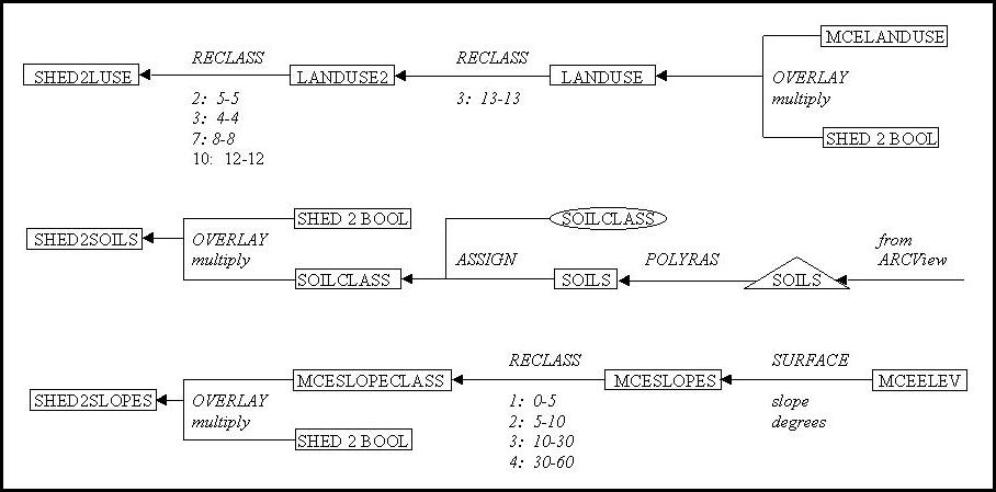
After deciding to use Watershed 2 for this project, I then proceeded to create the layers I was interested in for this particular watershed region.  The process of creating these layers is illustrated in the cartographic model above.

Landuse Layer
A simple overlay with the MCELanduse layer and the SHED 2 BOOL ("cookie cutter") layer produced a landuse image for the watershed of interest.  In the first reclass operation I changed the few lakes to forest cover because lakes are hydrological storage areas and can buffer the effect of increased runoff that occurs upstream.  This is difficult to model and the quantitative analysis is beyond my current understanding.  Since the project goal is to study a hypothetical drainage basin, this arbitrary change is completely reasonable.  The second reclass operation was a generalization of the original landuse classes.  The four classes that I did not have runoff coefficient data for were combined into other classes, preferably the ones to which they were most similar.

Soils Layer
First, the vector layer created in ARCView was imported back into IDRISI.  This vector layer was then rasterized.  The value of each zone was just its unique identifier.  I created an attribute value file that would assign each polygon a value of either 1 (open sandy loam), 2 (clay and silt loam) or 3 (tight clay).  This process was not random, as I made sure that the study region would have lots of variation.  This layer was then "clipped"  with the boolean image of the watershed to produce the final layer.

Slopes Layer
To avoid any possible error occuring along the boundary of the watershed, I applied the SURFACE module to the original DEM.  I used the module to produce a slope map, reclassed the values into ranges (according to the runoff coefficient data I had) and then clipped the image to the area of the watershed being studied.